R

The readr package

The readr package provides new functions for importing tabular data into R. Specifically, the functions read_table(), read_csv(), read_delim() are intended as fast (around 10 times faster) replacements for the base R read.table(), read.csv(), read.delim(). The readr functions do not convert strings to factors by default, are able to parse dates and times and can automatically determine the data types in each column (it does this by parsing the first 1000 rows). You can even import compressed files and they will be automatically decompressed and read into R. There is also file writing functionality, with write_csv(), write_tsv() and write_delim(). If you want even more speediness in your data importing, you might also consider the fread() function from the data.table package.

The readxl package

It used to be that the most reliable way to get data from Excel into R was to save it as a tab (or comma) delimited text file. While there are alternatives, such as the xlsx, XLConnect and gdata packages, that have other features (e.g. the ability to write excel files), if all you need is an easy way to import tabular data from xls and xlsx formats files, then the readxl package is for you. Importantly it has no external dependencies, so is very straightforward to install and use on all platforms. The syntax is very similar to the readr package functions, for example you specify the file name and the sheet of interest, read_excel("spreadsheet.xlsx", sheet = "data")

The haven package

The haven package provides functions for importing from SAS, SPSS and Stata file formats, read_sas(), read_sav()and read_dta(). This functionality is similar to that available in the base R foreign package but is often faster, can read SAS7BDAT files and formats, works with Stata 14 and 14 files. Following is the code to read SAS7BDAT.

install.packages("haven")
library(haven)
dat = read_sas("path to file", "path to formats catalog")

The returned object will be a data frame where SAS variable labels are attached as an attribute to each variable. When a variable is attached to a format in SAS and the formats are stored in a library, its path also needs to be supplied. Missing values in numeric variables should be seamlessly converted. Missing values in character variables are converted to the empty string. To convert empty strings to missing values, use zap_empty(), for example,

dat$x1 = zap_empty(dat$x1)

SAS, Stata and SPSS all have the notion of a “labelled”” variable. These are similar to categorical factor variables in R, but integer, numeric and character vectors can be labelled and not every value must be associated with a label. To turn a labelled variable into a standard factor R variable use the as_factor() function,

dat$facvar = as_factor(dat$facvar)

The haven package is under active development and becoming increasingly robust. If you have difficulties loading a file, try using the development version on GitHub:

devtools::install_github("hadley/haven")

For example, consider the National Youth Tobacco Survey (NYTS) from the CDC website.  After downloading the files (and installing the development version from GitHub) the data can be imported into R using

devtools::install_github("hadley/haven")
require(haven)
x = read_sas("nyts2014_dataset.sas7bdat","nyts2014_formats.sas7bcat")
# convert qn1 to a factor:
x$qn1 = as_factor(x$qn1)
View(x)

The rio package

The rio package describes itself as “a Swiss army knife for data I/O”. It unifies many of the above methods by providing the wrapper function import() that takes as an input the path to a data file. It then uses the file extension to determine the file type and imports the data into R. The one function can be used to import standard text files, RData, JSON, Stata, SPSS, Excel, SAS, XML, Minitab and many more. There is an analogous export() function that allows users to similarly easily export data to various file types.

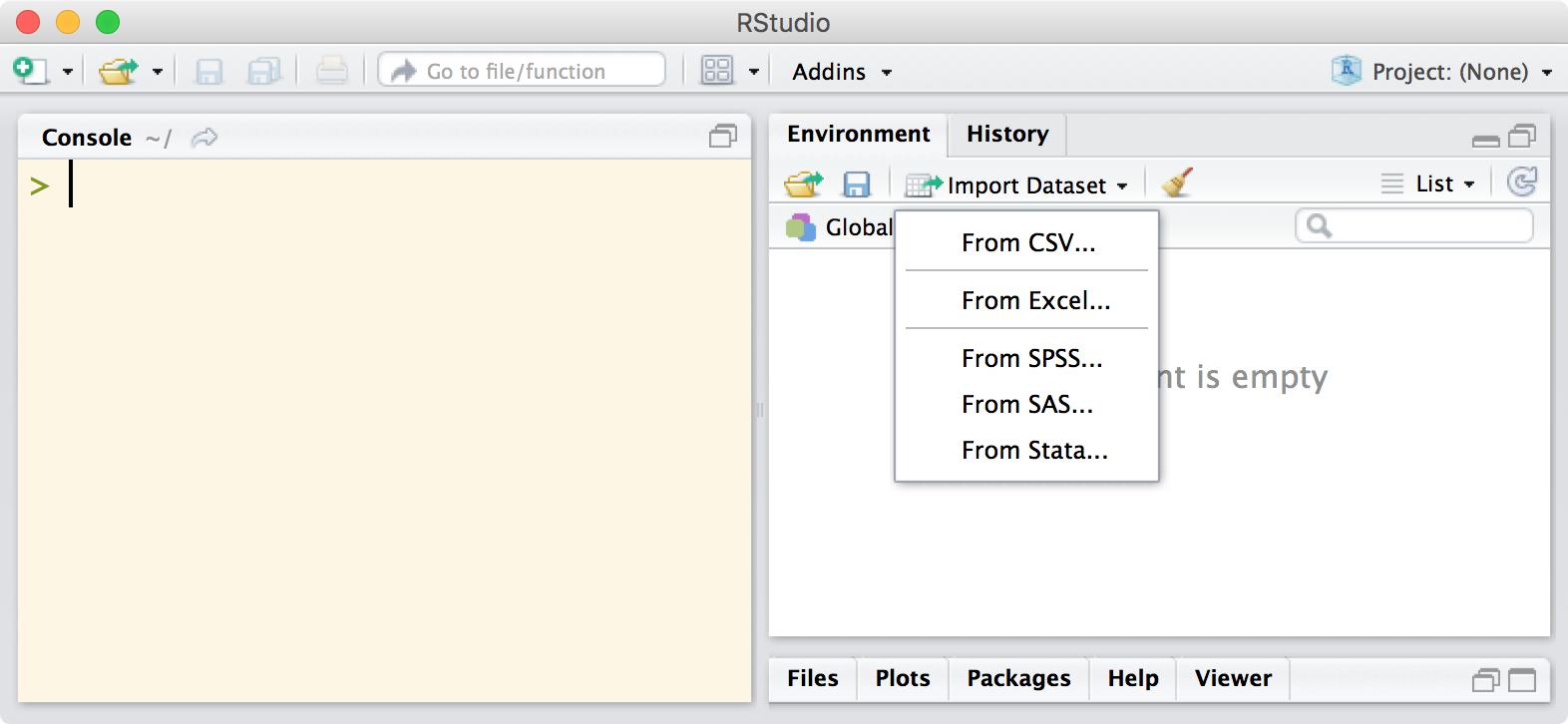
Using RStudio to import data

Recent versions of RStudio allow users to import various file types via a graphical user interface, which is perfect for novice users and experts alike as they get used to the new functions and customization options. Once you’ve clicked through the various options, it will output the required code at the console so that you can see exactly what was done to get the data in and edit the code as necessary for next time.

The team at RStudio have put together a webinar on getting data into R which is well worth watching.

Once you’ve got your data into R, you’ll probably need to restructure it in some way prior to analysis. To help with this, you may want to take a look at the tidyr package provides a suite of functions to get your data set in a standardized format, such that each observation is a row, each variable is a column and there are no data in the labels.

Getting started

The parallel package is part of base R which means that it’s already installed and you can’t find it on CRAN. You can load it in the usual way library("parallel"). The first thing you’ll want to do is detectCores() which checks how many cores you have available wherever R is running (probably your laptop or desktop computer).

Parallel apply

The family of apply functions (apply, lapply, tapply, sapply, etc.) in R provide an extremely convenient way of applying a function to the margins of an array, matrix, list, etc. If you’re using apply on a data frame, e.g. apply(X,2,median) to compute the median of the columns of X, you should consider using lapply instead because it’s much faster, e.g. lapply(X,median) which computes the median of each variable in the data frame X (there’s no need for a margin argument).

The apply functions operate serially, i.e. they calculate each value in sequence and are constrained to use only one of your computer’s cores. If you’re on a Unix-like system, the mclapply function is an easy way to distribute the computation across the available cores. To use mclapply, first code your calculations as a function that can be called with lapply. Make sure it works serially using lapply and then use mclapply to perform the computations in parallel.

library("parallel")
X <- data.frame(matrix(rnorm(1e+07), ncol = 200))
mclapply(X, median)

In this simple example, there is only a relatively minor speed improvement. To get the most out of parallel processes, the functions to be run in parallel should be non-trivial. There is an overhead associated with forking the process, so it is possible to slow your code down with mclapply if the time taken to send the tasks out to various cores takes longer than performing the task serially.

Windows can’t “fork” processes in the same way that Unix-like systems do. This means that you won’t see any improvements in speed when using mclapply on a Windows machine. On the plus side, your code won’t break – it will work as if you were simply using lapply. Microsoft has announced plans to incorporate a Ubuntu image into future releases of Windows 10 through a new infrastructure they’re calling “Windows Subsystem for Linux”. This means you may soon be able to run R in a native Unix-like environment (which supports forking and hencemclapply) on Windows 10 machines.

Parallel loops

An alternative to mclapply is the foreach function which is a little more involved, but works on Windows and Unix-like systems, and allows you to use a loop structure rather than an apply structure. To use foreach you need to register a “parallel backend”, for example using thedoParallel package. The doParallel package acts as an interface between foreach and the parallel package. A simple example of how this works is given below where we calculate a percentile bootstrap confidence interval for a least absolute deviations (LAD) regression parameter. In the code below, we resample a dataset 10,000 times and each time generate LAD regression coefficients.

library("quantreg") # for quantile regression function rq()
data(engel) # the data set we'll use
# help(engel) 
# plot(foodexp ~ income, data = engel)
# fit1 <- rq(foodexp ~ income, tau = 0.5, data = engel)
# abline(fit1)
library("foreach")
library("doParallel")
cl <- makeCluster(2) # create a cluster with 2 cores
registerDoParallel(cl) # register the cluster
res = foreach(i = 1:10000, 
              .combine = "rbind", 
              .packages = "quantreg") %dopar% {
  # generate a bootstrap sample              
  boot_dat <- engel
[sample(1:nrow(engel), replace = TRUE), ]
  # fit the model
  fit1 <- rq(foodexp ~ income, tau = 0.5, data = boot_dat)
  # return the coefficients
  fit1$coef
}
stopCluster(cl) # shut down the cluster

In the foreach() function we’ve specified that the results should be combined using rbind (i.e. the rows will be bound together, where the iththrow is the LAD regression coefficients from the ithth bootstrap sample) and we’ve indicated that the quantreg package needs to be loaded on each of the processes. The output is a matrix, that we’ve called res, which consists of two columns and 10,000 rows. We obtain a 95% percentile bootstrap by extracting the appropriate quantiles:

resdf <- as.data.frame(res)
quantile(resdf$income, probs = c(0.025,0.975), type = 1)

##      2.5%     97.5% 
## 0.4704510 0.6125974

The for loop syntax is very similar to a regular for loop in R, except it starts with foreach and uses the %dopar% function. If you use %do% instead of %dopar% evaluates the loop sequentially where one CPU will run at 100% until the job is finished. In the above example we asked for two cores to be used, hence with %dopar% both cores will run at 100% until the job is done. This means that a %dopar% loop running on two cores will finish in roughly half the time that it would have taken to run on a single core. As an example, the code above with 100,000 replications using%do% takes 3.0 minutes on my computer whereas using %dopar% takes only 1.6 minutes. It’s not exactly two times faster because of the computational overheads involved in sending the tasks out to the different cores and collating the results. For more details see the doParalleland foreach vignettes.

Distributed computing

The function mclapply can only use the cores of one machine, i.e. jobs can’t be distributed over several nodes of compute cluster. One way to do this in R is to use the parLapply function which can utilise the Message Passing Interface (MPI) system. For further details see the Rmpi package. The doMPI package provides an MPI parallel backend for the foreach package.

Other considerations

Parallel random number generation: When bootstrapping or performing simulation studies, it is desirable for each instance of R to generate independent, reproducible pseudo-random numbers. If there is an object .Random.seed in your R workspace that is then shared with the worker cores, all your instances of R may inavertently run identical simulations using identical “random” numbers. Alternatively, if .Random.seed is not in the workspace, then you will have independent streams of random numbers but it will not be reproducible. The parallel package includes a random number generator designed to overcome these issues. It can be enabled using RNGkind("L'Ecuyer-CMRG"). See the documentation of the parallel package for details.

Multi-threaded linear algebra computation: R can also be compiled against multi-threaded linear algebra libraries (BLAS, LAPACK) which can speed up calculations. One of the easiest ways to do this is to install Microsoft R Open (formerly known as Revolution R Open), however doing so ties you to a CRAN snapshot taken at a fixed point in time. You can still install the most up-to-date version of a package by manually specifying the repos argument.

Bioconductor: If you work with Bioconductor packages, you should look into BiocParallel which provides modified versions of functions optimised for parallel evaluation, tailored for use with Bioconductor objects.

So the next time you think about leaving a simulation running on your computer for the weekend, consider using mclapply instead of lapply or rewriting that for loop as a foreach loop and have it run overnight instead, or send it out to a supercomputer and have the results within a couple of hours!